Added: the following approach separates position steps and gradient steps,
from a digital filter point of view.
Put the pair of equations for momentum gradient descent:
$\qquad y_t = (1 + m) x_t - m x_{t-1} \ $ -- momentum, predictor
$\qquad x_{t+1} = y_t + h\ g(y_t) \qquad$ -- gradient
in a form with $y_t$ only, the points at which the gradients
$g_t \equiv - \nabla f(y_t)$ are evaluated:
$\qquad y_{t+1} = (1 + m)\, x_{t+1} - m\, x_t $
$\qquad \qquad = (1 + m)\, y_t - m\, y_{t-1} \ + \ (1 + m)\, h g_t - m\, h g_{t-1} $
$\qquad \qquad \approx Position\_filter( y_t, y_{t-1} ...; m_t ) $
$\qquad \qquad \quad + Gradient\_filter( g_t, g_{t-1} ...; h_t )\quad$ -- extrapolate ?
Why filters ?
There's a large body of digital filter know-how, which might give some insight.
For example, the 2-term extrapolator $1.9 x_t - 0.9 x_{t-1}$,
which is commonly used for both $Position\_filter$ and $Gradient\_filter$,
almost triples high-frequency noise [1 -1 1 -1 ...] .
So, use a longer, low-pass filter, matched to the noise.
(This may be naive; I'm no expert.)
Why separate filters for positions and for gradients ?
If $y_t$ and $g_t$ have very different noise patterns,
analyzing and controlling each one by itself
may be easier than doing both together.
Real gradients can be very noisy, so need smoothing,
either outside or inside the descent loop.
To see if filters are at all useful for momentum gradient descent,
we need examples and plots of real, noisy data,
before and after smoothing, on the web.
(Complete programs would be better, but cost time to put up;
start with files of $y_t$ and $g_t$, to filter and plot.)
Comments and links are welcome.
About the simplest case that makes sense to plot is 1d, here with $\nabla f(x) = x - 100$ .
1d is trivial, but shows how steps keep growing
until, for large values of momentum, they overshoot.
(It's also easy to play with gradient noise and gradient smoothing in 1d.)
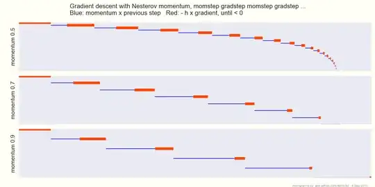
stepper: x - 100  momentum 0.5  h 0.1
...
15: x 96.5   + m 0.57   + g 0.29
16: x 97.4   + m 0.43   + g 0.22
17: x 98     + m 0.32   + g 0.17
18: x 98.5   + m 0.24   + g 0.12
19: x 98.9   + m 0.18   + g 0.093
20: x 99.2   + m 0.14   + g 0.07

stepper: x - 100  momentum 0.7  h 0.1
 1: x 0      + m 0      + g 10
 2: x 10     + m 7      + g 8.3
 3: x 25.3   + m 11     + g 6.4
 4: x 42.4   + m 12     + g 4.6
 5: x 58.9   + m 12     + g 2.9
 6: x 73.5   + m 10     + g 1.6
 7: x 85.3   + m 8.3    + g 0.65
 8: x 94.2   + m 6.2    + g -0.042

stepper: x - 100  momentum 0.9  h 0.1
 1: x 0      + m 0      + g 10
 2: x 10     + m 9      + g 8.1
 3: x 27.1   + m 15     + g 5.8
 4: x 48.2   + m 19     + g 3.3
 5: x 70.5   + m 20     + g 0.94
 6: x 91.6   + m 19     + g -1
The code, in outline:
x = x0
prevstep = 0
for iter in range( 1, maxiter+1 ):
    momstep = momentum * prevstep
    y = x + momstep
    gradstep = - h * gradfunc( y )  # h aka stepsize aka learning rate
    step = momstep + gradstep
    xnew = x + step
    print "%2d: x %-6.3g + m %-6.2g + g %-6.2g " % (iter, x, momstep, gradstep)
    if plot: ...
    if gradstep <= 0:  # back where we came from ?
        break  # restart
    x = xnew
    prevstep = step
Notice that this code is exactly the same with N-dimensional numpy vectors instead of scalars,
except for plotting, and restarting when gradstep <= 0.
For the latter, see no-U-turn restart.
See also: whats-the-difference-between-momentum-based-gradient-descent-and-nesterov on stats.stackexchange.


