Intuition for the Frobenius method

Question

I'm teaching a differential equations class now and I am hoping to give a reason for the Frobenius series method beyond simply "we guess these solutions". Now, for the Euler equation $$t^n x^{(n)}(t) + a_{n - 1} t^{n - 1} x^{(n - 1)}(t) + \dots + a_0 x(t) = 0$$ there is a good, easy explanation for why the fundamental solutions are of the form $x(t) = t^r$, where $r$ solves the indicial equation and repeated roots are handled by multiplying by powers of $\ln t$: just make the change of variables $s = \ln t$ and verify that this makes $t^n x^{(n)}(t)$ a constant-coefficient linear combination of the $x^{(k)}(s)$'s, and copy down the solutions to a constant-coefficient linear equation: $s^k e^{rs}$, with $k$ less than the multiplicity of $r$ as a root of the characteristic polynomial, which turns out here to be exactly the indicial polynomial.

But there isn't an apparent generalization of this analogy to arbitrary differential equations with regular singular points, $$t^n x^{(n)}(t) + a_{n - 1}(t) t^{n - 1} x^{(n - 1)}(t) + \dots + a_0(t) x(t) = 0,$$ with the $a_i(t)$ analytic around $t = 0$. You can make the same change of variables and render the equation non-singular, but it will:

1. still have variable coefficients;
2. even if you got the solutions as power series, the substitution $s = \ln t$ would make them into series in $\ln t$, which is not desirable;
3. when two roots differ by an integer then one of the solutions won't even be of the desired form;
4. when there's a repeated root, the second solution looks like $$x_2(t) = x_1(t) \ln t + x^r v(t),$$ where $v(t)$ is some other power series, anyway, which is not what you'd get from the change of variables in any obvious way. Now, it is true that there is the following relationship between $x_1(t)$ and $v(t)$: $$x_1(t) = \sum_{i = 0}^\infty b_i(r) t^{n + r} \qquad v(t) = \sum_{i = 0}^\infty b_i'(r) t^{n + r}$$ where we differentiate the coefficients with respect to $r$, considered somehow as a continuous variable.

So, my question:

Is there some connection, via a transform, change of variables, or approximation, that produces the Frobenius method by analogy with non-singular equations? Perhaps just when the roots of the indicial polynomial do not differ by integers?

Answer 1

Is there some connection [...] that produces the Frobenius method by analogy with non-singular equations?

When solving a differential equation by power series, you assume that your solution can be expressed as a power series (which is quite reasonable assumption, since many analytic functions can be expressed that way). You can substitute the power series into your equation and find the expression for the coefficients.

This works quite well when your variable coefficients of the derivatives are "nice" functions. But when they have some singularities, there's a problem with that approach: when you substitute your power series and simplify, you'll come to something in the lines of

$$(\mbox{some expression with n})\cdot a_n = 0$$

and you find out that you cannot make the expression in the parenthesis to be $0$ for any value of $n$, which implies that it is $a_n$ which must be $0$. But this gives us just a finite power series (that is, a polynomial); or, what's worse, you have all coefficients equal to zero, but this is just the trivial solution $y = 0$. It is correct, but not much of our interest.

The reason why we cannot get some nice power series in this case is that our assumption was wrong: what mathematics is trying to tell us here is that the solution function cannot be expressed by simple power series when it has singularities, because then you have some negative powers of $x$ involved (which means division by $0$ when $x=0$), or even fractional powers (roots, which don't have values for some numbers) or real or complex powers.

Enter the Frobenius method.

This can be easily fixed by assuming something more: that our power series is multiplied by $x^r$, where $r$ can be any real or complex exponent. This part of the solution accounts for the non-natural powers of $x$ in our solution. So we have the ansatz (trial solution):

$$y(x) = x^r \sum_{n=0}^\infty a_n x^n$$

which we can rewrite simpler as:

$$y(x) = \sum_{n=0}^\infty a_n x^{r+n}$$

When you substitute this trial function into your equation you'd get the indicial equation from which you can determine the value(s) of your exponent $r$.

Edit: I added answers for your follow-up questions to clarify it somewhat more.

Why should multiplying by this weird power help?

As I've said, some functions are not "nice". They have singularities (e.g. divisions by zero, discontinuities etc.). Then, they cannot be expressed as simple power series such as

$$y = \sum_{n=0}^\infty a_n x^n$$

because they don't have natural exponents in their powers. Their powers can be negative (division), fractional (root extraction), or even some real or complex exponents. So we need to modify our power series to account for such "weird" exponents. We do that by adding (or subtracting) some other constant $r$ to (from) our exponent $n$:

$$y = \sum_{n=0}^\infty a_n x^{n+r}$$

Although $n$ could be only some natural number, $r$ can now be any number (even a complex number), and we would have to determine what number it is (sometimes there will be more than one answer for that question). That's what indicial equation is for.

But before that, we shall notice something: After adding/subtracting $r$ to/from the exponent, this is no longer a standard power series (its exponent can now be non-natural). But we can use the rules for exponents to extract this $r$th power of $x$

$$y = \sum_{n=0}^\infty a_n x^n x^r$$

and then move out of the sum since this is a common factor of all its terms:

$$y = x^r \sum_{n=0}^\infty a_n x^n$$

and we have our original power series back, but we note that it is now multiplied by some power of $x$. And this is the answer to your question why do we multiply the trial series by $x^r$.

If a power series should occur, is there any relationship with the series solutions to constant-coefficient equations?

Yes there is. For constant-coefficient equations the solution was in a form:

$$ y = C_0 e^{r_1 x} + C_1 e^{r_2 x}$$

where $r_x$ and $r_y$ were roots to the "characteristic equation" (or "indicial equation"). You could get the same answer with simple power series, since constant coefficients are "nice" functions (analytic) too. You'd get a pattern in the coefficients of the power series, with factorials in there, which indicates the exponential function, and this is indeed the solution. If you have some pattern-matching skill, you can try restoring the original function (exponential in this case) from the power series. Been there, done that, this is perfectly possible.

In the case of variable-coefficient equation such as Cauchy-Euler (or equidimensional) equation, we are told that the solution is in a form:

$$y = C_0 x^{r_1} + C_2 x^{r_2}$$

which doesn't seem like the exponentials we are familiar with from the constant-coefficient equations. But note that you can rewrite $x$ as $e^{\ln x}$, and when you substitute it to the solution pattern you'll get:

$$y = C_0 (e^{\ln x})^{r_1} + C_2 (e^{\ln x})^{r_2}$$

and using the laws of exponents we see that:

$$y = C_0 e^{r_1 \ln x} + C_2 e^{r_2 \ln x}$$

and this form might look more familiar, since there is a sum of exponentials again. But now we use natural logarithms of $x$ instead of $x$ directly.

The ansatz approach is certainly motivational, but it's not intuitive and gets less satisfying the more you learn.

Well, intuition is also something you learn. For you this might not be intuitive, but when you gain experience and learn some patterns, you'd start to notice them in your equations when they appear again and again, and they'll become intuitive to you then.

These questions can't be answered by ansatz, which students always interpret as "guess and check", which it sort of is.

It's not much "guessing", it's rather an "educated guess", or "intelligent heuristics". You don't guess just anything ─ you use what you know for your guess. For example, when you have simple equation like this:

$$y' = k y$$

you can think in these lines:
"What function $y$ is proportional to its own derivative?" There is only one such function: the exponential, $y = e^x$. But we want a function which derivative will be proportional to that function in a certain ratio, a certain constant of proportionality, which is $k$. If you know that $\left(e^{kx}\right)' = k e^{kx}$, then you can guess the correct solution right away. But if you don't, you can leave some constant "to be determined later" in your trial solution, and put it into the equation to see what will happen and what value that constant shall have for the equation to be satisfied.

It happens that the exponential function solves any linear differential equation, and this is not a coincidence: The exponential is the eigenfunction (or proper function) of differentiation. This means that when you apply differentiation to it, it will come out untouched, but sometimes multiplied by a constant (which is then an eigenvalue; in the case above it was $k$). So this is not much a "guess" when you try to use exponential for other similar equations to see if it still fits. If from some reason it won't fit, you'll loose nothing: Mathematics will tell you that your assumption was wrong, and sometimes you can notice what needs to be improved to get the correct answer. For example, you need some power of $e^x$ (which is $e^{kx}$ as in our example above). Or you need to multiply by $x$, or some power of it (as $x^r$ in our example with Frobenius series).

Same goes with variable-coefficient equations, like Cauchy-Euler equation. You can see that there's a power of $x$ at every derivative, and this power of $x$ has the same degree as the order of the derivative. Recall that when we differentiate some power of $x$, its exponent drops down by 1 and it goes as a constant multiplier. But then there's that variable coefficient which is also a power of $x$, so multiplying our derivative by it will raise the power back. And since the degree of that power is the same as the order of the derivative, whatever it went down in differentiation, it will go up back again to the same level. So we will have the same powers of $x$ everywhere (a common factor!), just multiplied by some constants, which we can always tweak in a way to turn the whole equation to 0. So substituting $x^n$ into the equation as your trial function isn't that bad idea in this case. And, as you can see, you can deduce what function will work from the form of the equation, by observing what these derivatives will do with it, and how can you make the whole equation cancel.

Answer 2

As you note, Ryan, it is quite sensible to try power functions for the Euler equation. Now the general equation with regular singular points is an analytic deformation of the Euler equation (near each of those singular points), in that its coefficients are analytic functions which, when evaluated at 0, give you an Euler equation. It is therefore very natural to look for solutions which are deformations of the solutions of the Euler equation. That is precisely what the Frobenius method does.

And it works marvels. For example, the indicial equation of the general equation is precisely the same as that for the corresponding Euler equation, so that the behaviour of solutions is qualitatively the same as for the Euler equation.

Answer 3

Overview

I will add three different points of view to those in other answers. The OP already makes some important observations, but to make this answer self-contained, I will repeat some of them. The three points of view mainly rest on formal algebraic properties of differentiation, and analytical questions about convergence are left aside, as they are well-established. We will emphasize in particular how non-integer powers arise, how powers of logarithms arise in analogy to linear systems with constant coefficients, and why powers of logarithms arise only sometimes in the case of roots differing by an integer. I will include remarks that I think might be helpful in discussing the Frobenius method with students.

A review of equidimensional operators, that is, ones of the form $L=\sum\limits_{k=0}^n \alpha_k t^k {d^k \over dt^k}$, will show a more uniform approach to series solutions in powers of $t$, whether Frobenius or standard integer-power series. The differences emphasized in textbooks come from properties of the linear system that determines the coefficients, most importantly the kernel of $L$. This will also give the generalization of the OP's explanation of the solution to the Euler equidimensional equation that the OP seeks. If you do not know this already, it will be a surprise that the non-singular case corresponds to:

the case of indicial roots differing by an integer.

The OP alludes to a result of Frobenius in point 4, and since Frobenius's approach has not been mentioned, I will give a brief review. He constructs a function that almost solves the differential equation, depending on a parameter $r$ (as the exponent of $t^{r}$). He then determines values of $r$ for which it is a solution. It is beautiful lesson in problem-solving. It also gives a different explanation for the source of $\log t$ in the solutions, different from the linear-algebra explanation we will give first.

Finally, there are roots of Frobenius's method in first-year calculus that are sometimes overlooked (for pedagogical reasons). For instance: (1) How do logarithms arise? Or (2) the series that stand out are Taylor series; but Frobenius-type series have the same theory of radius of convergence as Taylor series and can be expanded in a similar way. And (3) we can connect series expansions of solutions of differential equations to a standard method of development that applies to both power and Frobenius-type series. The hope is that seeing the connections builds a coherent picture from which an intuition may spring.

We will assume throughout, as in the OP, that $t=0$ is an ordinary point or a regular singular point. I will use "power series" only in the case where the exponents are nonnegative integers; I will use "series of powers" when the exponents differ by integers but themselves may or may not be integers.

Summary of points for building an intuitive picture

I will put a bulleted summary in front, because this is the internet.

• Powers are alike: The power rule implies that the substitution of a series of powers $x = \sum_s c_s t^s$ into in a suitably nice linear differential equation $\Omega[x]=0$ leads to a sequence of triangular linear systems. The summation is over $s=r,r+1,\dots$, where $r$ might be an integer or other complex number. The restriction on $r$ comes from the indicial polynomial of $\Omega$. When $t=0$ is an ordinary point, then $r$ must be a nonnegative integer and the series will be a traditional power series.
• Equidimensionality is key: The equidimensional operator $t {d \over dt}$ maps not only $t^s$ to a constant times $t^s$ but also $p(\log t)\,t^s$ to $q(\log t)\,t^s$, where the polynomials $p$ and $q$ have the same degree. A convenient basis of functions for general equidimensional linear operators is $\{\,(\log t)^j t^s\,\}$, $j$ a nonnegative integer, for each power $s=r,r+1,\dots$ where $r$ is an indicial root for $\Omega[x]=0$. An upper bound on the exponent $j$ may be taken to be one less than the differential order of $\Omega$.
• The differential equation $\Omega[x]=0$ in which $t=0$ is an ordinary point or a regular singular point is equivalent to one of the form $L[x]=R[x]$, where $L$ is equidimensional and the $t^s$ component of $R[x]$ is determined by lower-degree terms in the series for $x$. The indicial polynomials of $L$ and $\Omega$ are the same.
• A nontrivial kernel is another key: We have $L[t^s]=I(s)\,t^s$, where $I(s)$ is the indicial polynomial. It is of deficient rank when $s$ is an indicial root. This is at the heart of the cases of repeated roots and of roots differing by an integer, and why powers of $\log t$ appear in solutions.
• The indicial roots for an ordinary point are consecutive nonnegative integers starting with $r=0$. From a Frobenius series point of view, it is remarkable that the solutions are pure power series and have no $\log t$ components. This happens because for the corresponding operator $R$, the series for $R[x]$ has its initial coefficients equal to $0$, up to one less than the differential order of $\Omega$.
• Frobenius's series $x_r$ interpolates between solutions that start at powers $r=r_1,r_2,\dots$. The exponent $r$ is a good interpolating parameter because for any $r$ and equidimensional operator, $t^r$ is an eigenfunction.
• When $\Omega[x_r]$ vanishes to high order, its derivatives ${\partial^i \Omega[x_r]/\partial r^i}$ also vanish up to a certain order.
• The differentiation of $t^{r+k}$ with respect to $r$ yields $\log t$ factors. The ability to differentiate and get a solution is connected to the multiplicity of the roots of the indicial polynomial $I(r)$ or of $(r-r_2)\,I(r)$ in the case of roots separated by an integer.
• The integration of powers yields not only powers but logarithms, and so solving differential equation in terms of series of powers yields logarithms, too.

Maybe the summary is enough for you. Some more details follow.

Equidimensional operators

Foreword: I explain in terms of linear algebra, because I think that makes it clearer to teachers; for students, second-order equations could be explained in terms of explicit linear equations, which they will be accustomed to from power series solutions.

An equidimensional operator leaves invariant the vector space $E_s^j$ of dimension $j+1$ consisting of the functions $p(\log t)\,t^s$, for all polynomials $p$ of a fixed maximum degree $j$ and a fixed complex number $s$. One can make the case that since $d(\log t)=dt/t$ is dimensionless, so is $\log t$; thus all the terms in $p(\log t)\,t^s$ have the dimensions of $t$ raised to the $s$. For most powers $s$, $L$ is an isomorphism. For some powers $s=r$, $L$ has a nontrivial kernel. These powers are indicial roots. For these powers $L$ maps $p(\log t)\,t^r \mapsto q(\log t)\,t^r$, where $\mathop{\text{deg}}q<\mathop{\text{deg}}p$. In fact, $L$ maps $E_r^j$ surjectively onto $E_r^{j-\kappa}$, where $\kappa$ is the dimension of the kernel of $L$.

In the OP, the differential equation is given in the form $\Omega[x]=0$, where $$\Omega[x] = t^n x^{(n)}(t) + a_{n - 1}(t) t^{n - 1} x^{(n - 1)}(t) + \cdots + a_0(t) x(t) \,.$$ with coefficients $a_k(t)$ which are analytic in a neighborhood of $t=0$. Let $L$ be the equidimensional linear differential operator $$L[x] \equiv t^n x^{(n)}(t) + \alpha_{n - 1} t^{n - 1} x^{(n - 1)}(t) + \cdots + \alpha_0 x(t) \,,$$ where $\alpha_k = a_k(0)$. Finally let $$R[x] = -\bigl[(a_{n - 1}(t)-\alpha_{n-1})\, t^{n - 1} x^{(n - 1)}(t) + \cdots + (a_0(t) - \alpha_0)\, x(t)\bigr] \,,$$ so that the coefficients $a_{k}(t)-\alpha_{k}$ are analytic and vanish at $t=0$. Thus $\Omega[x]=0$ is equivalent to $L[x]=R[x]$.

Solution procedure

Task: To solve the differential equation $L[x] = R[x]$.

Below, $E_s^j$ is to taken be a subspace of $E_s^{n-1}$, where $n$ is the differential order of $L$ as above. We then develop a series solution as follows. Let $x = \sum_s p_s(\log t) t^s$, where the "coefficient" $p_s(\log t)$ is a polynomial in $\log t$ of degree at most $n-1$ and the summation is over a sequence of indices $s=r, r+1, r+2,\dots$. We will solve degree by degree for the coefficients of $p_s$ from a linear system derived from the $t^s$ components of $L[x] = R[x]$. The $t^s$ components of $R[x]$ are, by the hypotheses on $R$, determined by the lower-order terms of $x$; the initial power is a special case treated below. It may be possible to find the general solution of each linear system over $E_s^0$, which case we will have a Frobenius series without $\log t$ terms in it. If $L$ has a nontrivial kernel on $E_s^{n-1}$, then the solution of the $t^s$ component lies in a subspace $E_s^j$. When $j > 0$, the general solution may have powers of $\log t$; indeed, it will have powers of $\log t$ when $s=r$ is the initial power and $r$ is a repeated root.

Initial power $t^r$. We can start the series at an indicial root because $L[t^r] = 0$ and the $t^r$ component of $R[x]$ is $0$ because of the assumptions on its coefficients. The solution space is $\mathop{\text{ker}} L = E_r^{\mu-1}$, where $\mu$ is the multiplicity of the root $r$. If $\mu>1$, the general solution will have powers of $\log t$ up to the power $\mu-1$.

Subsequent powers $t^s$. Then proceeding degree by degree, we can solve the system $L[x] = R[x]$ at each power $t^s$. When $s$ is not an indicial root, $L$ is an isomorphism on $E_s^j$ for all $j$, the solution will not introduce higher powers of $\log t$. When $s$ is an indicial root, $L$ is not an isomorphism; this is the case where indicial roots differ by an integer. Let's say the $t^s$ component of $R[x]$ lies in $E_s^j$. Then $L$ maps $E_s^{j+\kappa}$ onto $E_s^j$, where $\kappa$ is the dimension of the kernel of $L$ (on $E_s^n$). The general solution to the $L[x]=R[x]$ at the power $t^s$ will lie in a subspace of $E_s^{j+\kappa}$. This may lead to the degree of $p_s$ increasing up to $j+\kappa$.

Questions and answers

Why do ordinary points give ordinary power series solutions?

Power series development at ordinary points may be subsumed under the Frobenius method. For an ordinary point, one has $x^{(n)}(t) = \sum\limits_{k=0}^{n-1} a_k(t) x^{(k)}(t)$, where the $a_k(t)$ are analytic, but do not necessarily vanish, at $t=0$. Multiplying by $t^n$, we can write the differential equation in terms of the equidimensional operator $L = t^n{d^n \over dt^n}$, that is, $L[x]= t^n x^{(n)}(t)$. We have for the right-hand side $R[x]=\sum\limits_{k=0}^{n-1} t^n a_k(t) x^{(k)}(t)$, which vanishes to at least order $n$ at $t=0$. The indicial roots of $L$ are sequential integers, $r=0,1,2,\dots,n-1$, each of which gives a series in nonnegative powers of $t$, possibly with a $p(\log t)$ coefficient. However, $L[t^s]$ and the $t^s$ component of $R[x]$ are both zero for $s=0,1,\dots,n-1$. Thus the coefficients of the series of $x$ are free variables up to the power $t^{n-1}$, and no powers of $\log t$ are introduced.

Why do repeated roots always have $\log t$ components and roots differing by an integer only sometimes?

This has been answered above, but I will be more explicit. Let $r$ be an indicial root and suppose we are solving for the series that begins at the power $t^r$. If the multiplicity of the root is $\mu=1$, then the general solution is $E_r^0$ and there are no $\log t$ terms (the polynomial $p_r$ is a free constant); if $\mu > 1$, then the general solution is $E_r^{\mu-1}$ and there are logarithmic terms up to the power $(\log t)^{\mu-1}$. Subsequently, when we run into a power $s=r_1$ that is an indicial root (thus $r_1-r$ is an integer), $L$ has a kernel of dimension $\kappa$ equal to the multiplicity of the root $r_1$. Suppose the $t^s$ component of $R[x]$ lies in $E_s^j$. Then the general solution will lie in $E_s^{j+\kappa}$ and be of the form $p_{r_1}(\log t)\,t^{r_1}$, where $p_{r_1}$ has, say, degree $m \le j+\kappa$. If $m$ is greater than the degree of $\log t$ in the $t^{r_1}$ component of $R[x]$, then $L[x]=R[x]$ determines the leading coefficient of $p_{r_1}$. In general, as we proceed to higher powers, $L$ acts on $(\log t)^m t^s$ by multiplying it by $I(s)$ (and adding lower degree terms). Solving for the coefficient of the leading term results in solving the same equation as for the solution $x_1$ starting at the root $r_1$. Thus we obtain a multiple of $(\log t)^{m}$ times the solution $x_1$ as part of the solution. In the textbook case of a second-order differential equation, this means a solution of the standard form, with the constant $\beta$ possibly being zero: $$x(t) = \beta\, x_1(t) \log t + \sum_{n=0}^\infty b_n t^{r+n} \,.$$

Are power series more natural than Frobenius and why in both kinds do the powers differ by integers?

This is probably obvious to many, but first an example. From the exponential Taylor series, the series for $x_1=\exp\left(\sqrt{t}\right)$ has powers that differ by $1/2$, not by integers, and $x_1$ is a solution to $4 t x''+2 x'-x=0$. So perhaps one ought to explain why half-integer steps do not seem to occur in Frobenius/power series expansions. The obvious reason for integer steps is the power rule, which changes powers by $1$. In fact, one feels that the half-integer-step series for $\exp\left(\sqrt{t}\right)$ is best viewed as the sum of two integer-step series, one that begins at $t^0$ and one that begins at $t^{1/2}$. Indeed, that is how the Frobenius series would be constructed, since $0$ and $1/2$ are the indicial roots. It's a different matter when the difference in powers is irrational, like $\exp\left({t}^{\sqrt{2}}\right)$. Fractional calculus can help, I suppose, but we'll leave that aside. A teacher could use such an example to suggest that Frobenius series are not quite at the edge of how strange series of powers can be.

Connection to autonomous linear differential equations

A lot of the theory of linear differential operators with constant coefficients, $A=\sum\limits_{k=0}^n \alpha_k {d^k \over dz^k}$, and equidimensional operators translate back and forth via the substitution $t = e^z$. For instance multiplying a power $t^r$ by $\log t$ that occurs with repeated roots corresponds to multiplying $e^{r z}$ by $z$. Powers $t^s$ are eigenfunctions of $t {d \over dt}$, and correspondingly exponentials $e^{s z}$ are eigenfunctions of ${d \over dz}$. The principal difference is that series in powers of $t=e^z$ are quite different than series in powers of $z$. I don't think I have ever seen a solution to an differential equation in terms of a series in $e^{s z}$, other than Fourier series, which is different. For this reason, the problem with roots differing by an integer, that is, with $e^{r z}$ and $e^{(r+N)z}$, does not arise, unless.

Summary

To me, to describe the Frobenius method as multiplying a power series by an arbitrary power makes power series appear a natural choice and Frobenius series seem weird. There are reasons why we look at series this way, based in history and the standard curriculum. However, framing Frobenius series this way is misleading, imo. When a series $\sum_s c_s t^s$ has powers $s$ that pairwise differ by an integer, the power rule leads to a linear system for the coefficients in a linear differential equation, whether or not $s$ runs through integers. Certain conditions on the differential equation ensure the system is solvable. There is nothing special beyond these conditions about $s$ being a nonnegative integer from an algebraic point of view. Of course, a more general basis $\{ (\log t)^j t^s \}$ leads to a greater range of functions that may be represented. This is probably clear to most, but perhaps not to all students who are just learning how mathematics works. I hope I have not tried your patience by mentioning possibly obvious remarks that are helpful to have at hand in discussions with curious students.

Exercises

<sub>1. Show that $L$ operating on $x=(\log t)^j t^s$ equals $I(s) (\log t)^j t^s$ plus lower powers of $\log t$, where $I(s)$ is the indicial polynomial of $L$.
2. Show further that $L$ operating on $x=(\log t)^j t^s$ equals $I(s) (\log t)^j t^s + j\,I'(s) (\log t)^{j-1}$ plus lower powers of $\log t$, if $j \ge 1$.
3. Generally, $L$ operating on $x=(\log t)^j t^s$ equals $\sum\limits_{i=0}^j {j \choose i} I^{(j-i)}(s) (\log t)^i t^s$.
3. The dimension of the kernel of $L$ operating on $x=(\log t)^j t^s$ equals $\sum\limits_{i=0}^j {j \choose i} I^{(j-i)}(s) (\log t)^i t^s$.
4. The function $t^r$ is an eigenfunction of $t {d\over dt}$ with eigenvalue $r$.
5. Under the substitution $t=e^z$, the function $t^r$ becomes the eigenfunction $e^{rz}$ of ${d\over dz}$ with eigenvalue $r$.
6. Under the substitution $t=e^z$, the equidimensional operator $L$ is transformed into a linear differential operator $M$ with constant coefficients, and the indicial polynomial of $L$ and the characteristic polynomial of $M$.
7. Let $\Lambda_r$ be the equidimensional operator $t {d\over dt} - r$. Show that $L$ is the product over the indicial roots $r$, counting multiplicity, of the operators $\Lambda_r$. (This corresponds to $M$ in the previous problem being a product of the operators ${d\over dz} - r$ over the characteristic values $r$.)
8. Given a function $x(t)$ with a Frobenius series representation, how to find $r$, the power of $t$ in the leading term?
9. Let $\phi = \left(1+\sqrt{5}\right)/2$ be the golden ratio. Show that $x(t) = t^\phi + \sum_{k=-\infty}^\infty {1 \over |k|!} t^{k+\phi}$ is a solution to $\left(t^2+1\right)t^3x''-\left(t^4+2\phi\,t^3+2(\phi-1)\,t-1\right)t\, x'+\left(\phi\,t^4+2\phi\,t^3-2t^2-\phi\right)x=0$. (Note that $t=0$ is an irregular singular point; apparently they can have series solutions that are infinite in both directions.)</sub>

Frobenius's approach

The OP alluded to a result of Frobenius in point 4 but did not mention Frobenius's approach explicitly. Frobenius's derivation gives another viewpoint, one that shows how the $\log t$ components arise out of basic calculus.

Frobenius's approach is to solve the recurrence relations for the series solution to the differential equation $\Omega[x]\equiv L[x]-R[x]=0$ beginning at an arbitrary $r$, where $r$ may vary continuously. Thus we have a series $x_r = \sum_{n=0}^\infty c_{r+n} t^{r+n} = t^r\sum_{n=0}^\infty c_{r+n} t^{n}$ that is not necessarily a solution to the differential equation; however, $c_{r+1},c_{r+2}\,\dots$ formally satisfy the recurrence relations arising from the differential equation, and $c_r$ is an arbitrary constant, which for convenience we will take to be $c_r=1$. There is an obstruction to solving the recurrence relations when for some $n$, $r+n$ is an indicial root, which we will address later. For now, assume $r+n$ is not an indicial root for any positive $n$. Again let $I(r)$ denote the indicial polynomial. Then $\Omega[x_r]= I(r)\,t^r$, the higher degree terms canceling out by construction. If $r_1$ is an indicial root and no $r_1+n$, $n$ a positive integer, is also an indicial root, $x_{r_1}$ will be a solution. If $r_1$ is a repeated root, then $I(r_1)=I'(r_1)=0$. Thus $\Omega\left[{\partial \over \partial r}x_r\right]={\partial \over \partial r} \Omega[x_r]= I'(r) \cdot t^r + I(r) \cdot {\partial \over \partial r} t^r $, which vanishes at $r=r_1$. Therefore, ${\partial x_r / \partial r} \big\vert_{r=r_1}$ is a solution to the differential equation. It may be written in the form $$\eqalign{ {\partial \over \partial r}x_r \bigg\vert_{r=r_1} &= \left({\partial \over \partial r} t^r \right)\sum_{n=0}^\infty c_{r+n} t^{n} + t^r\left({\partial \over \partial r} \sum_{n=0}^\infty c_{r+n} t^{n} \right) \bigg\vert_{r=r_1} \cr &= t^r(\log t)\, x_r + t^r \sum_{n=0}^\infty {\partial c_{r+n}\over \partial r} t^{n} \bigg\vert_{r=r_1} \,. \cr }$$ If the multiplicity of the root is $j$, then ${\partial^i x_r /\partial r^i}\big\vert_{r=r_1}$, $i=0,1,2,\dots,j-1$, are all solutions with terms that have factors that are powers of $\log t$ from degree $0$ to $i$.

Now suppose $r_2$ is an indicial root and $r_1=r_2+N$ is also a root for some positive integer $N$. The procedure is somewhat intricate to summarize, and I hope have made the following clear enough. For simplicity, suppose $r_2$ and $r_1$ are simple roots and no other root differs from $r_2$ by an integer. Then $x_{r_1}$ is a Frobenius series solution as above. Let's consider solving for the coefficient of the $t^s$ term in the series for $x_r$, where $s$ is $r+k$ for some positive integer $k$. We have $L[c_s\,t^s]=c_s I(s)\,t^s$, and we set it equal to the $t^s$ term of $R[x_r]$; let the term be $\rho(s)\,t^s$. Thus $c_s I(s)= \rho(s)$, and $c_s = \rho(s)/I(s)$ may have poles at the indicial roots. If $\rho(s)$ vanishes as $s \rightarrow r_1$ (equivalently $r \rightarrow r_2$), then $c_{r_1} = \lim\limits_{s \rightarrow r_1} c_s$ will exist since we are assuming $r_1$ to be a simple root of $I(s)$, and $x_{r_2}$ will be a solution. If $\rho(s)$ does not approach $0$ as $s \rightarrow r_1$, the $c_s$ will have a simple pole. The scalar multiple $x=(r-r_2)\,x_r$, where $r-r_2$ is the difference in $s=r+k$ at $r=r$ and $r=r_2$, satisfies the recurrence relations for powers $s>r$. The series $x$ will have a coefficient of $t^{s}$ that does not have pole, but will approach a limit, as $r \rightarrow r_2$. Therefore the limit of $x=(r-r_2)x_r$ will be a solution; in fact, it approaches $\beta \,x_{r_1}$ where $\beta$ is the limit of $(r-r_2)\,c_{r+N}$. (The factor $r-r_2$ annihilates the coefficients of $t^s$, $s<r_1$, in the limit, and the recurrence starts afresh with $c_{r_2}=\beta$.) Then $\Omega[(r-r_2)\,x_r]=L[(r-r_2)\,x_r]=(r-r_2)\,I(r)$ has a double root at $r=r_2$, which is the critical result we need. Therefore $$\Omega\left[{\partial \over \partial r}(r-r_2)\,x_r\right] = {\partial\Omega[(r-r_2)\,x_{r}] \over \partial r} = 0 \quad\text{at}\ r=r_2 \,.$$ Thus we get a solution, that is the limit of the following as $r \rightarrow r_2$: $$\eqalign{ {\partial \over \partial r}(r-r_2)x_r &= \left({\partial \over \partial r} t^r \right)\sum_{n=0}^\infty (r-r_2)\,c_{r+n} t^{n} + t^r\left({\partial \over \partial r} \sum_{n=0}^\infty (r-r_2)\,c_{r+n} t^{n} \right) \cr &\rightarrow \beta\,x_{r_1} \log t + t^{r_2} \sum_{n=0}^\infty \left({\partial \over \partial r}(r-r_2)\,c_{r+n}\Big\vert_{r=r_2}\right) t^{n} \,, \cr }$$ where $\beta$ may be $0$.

If $r_2$ has multiplicity $j$, then let $x = (r-r_2)^{j-1} x_r$ and differentiate up to $j-1$ times to get solutions with corresponding powers of $\log t$. When there is another indicial root $r_3$ separated from of the others by integers, multiply by an appropriate power of $r-r_3$, and so forth.

Successive integrations

Using successive integration to solve $y' = f(x, y)$ goes back well before Picard, perhaps beginning with Newton in 1670/71, who used it to develop power series solutions (see image below). When distilled to its basic algebraic recipe, it becomes the standard method of solving recurrences for the coefficients. The recurrence relations encode the integral power rule. While Taylor developed his series from the theory of interpolation, a common way now is to recursively integrate by parts. It's not the same as solving differential equations with the methods of Newton or Picard, but similarly, each integration adds the next power to the series development via the power rule. While it's taught in calculus only with integer powers, the procedure works on functions like $(\sin t)/\sqrt{t}$, if you start with the ${1/2}$ power, to obtain a Frobenius-like series. The integral remainder may be used to show convergence. If this were already in the student's experience, the Frobenius method would seem less strange.

To connect the remark on recurrences and integration to $\log t$ in Frobenius's method, consider the integration of powers. If we integrate powers and potentially any power may arise, then we will have to integrate $1/t$; and when we integrate successively, we will integrate $\log t$ repeatedly, which has the form $A\,t^{n} \log t + p(t)$, where $p$ has degree $n$. First, I would be surprised if any calculus student thought the appearance of $\log t$ in the integration of powers unremarkable. Second, if this occurs in successive integration, the series formed will look like a Frobenius series solution for a repeated indicial root. So one can connect the appearance of $\log t$ in the integration of powers to Frobenius solutions.

It seems easiest to explain how successive integration of an equidimensional operator through a example, a simple one chosen to illustrate how $\log t$ arises from repeated integration when $r$ is a repeated root. Let $\Lambda_r$ be the equidimensional operator $t {d\over dt} - r$. Our integration will be the inverse of this operation, similar to the way antiderivatives are the inverse of $d/dt$. Let's solve $L[x]=R[x]$ when $L = \Lambda_r^2$ and $R[x] = R_1[\Lambda_r[x]]$, where $R[y] = a(t)\,y$ with $a(t)$ analytic at $t=0$ and $a(0)=0$ as before. By inspection, one can see $x_1(t)=t^r$ is a solution, since $\Lambda_r[t^r]=0$, but let's start from the beginning. To get a complete solution, we'll first integrate $\Lambda_r[y]=R_1[y]$ and then $\Lambda_r[x]=y$. $$\eqalign{ t {dy \over dt} - r\,y &= (a_1 t + a_2 t^2 + \cdots)\,y \cr t {dy \over dt} &= (r + a_1 t + a_2 t^2 + \cdots)\,y \cr \int {dy \over y} &= \int\left({r \over t} + a_1 + a_2 t + \cdots\right) dt \cr \log y &= r \log t + a_1 t + {\textstyle{1\over2}} a_2 t^2 + \cdots) + C \cr y &= c_1 t^r \exp\left(a_1 t + {\textstyle{1\over2}} a_2 t^2 + \cdots\right)\cr y &= c_1 t^r \sum_{k=0}^\infty b_k t^k\cr }$$ We will apply an identity for $\Lambda_r x$ in the second integration: $$t {dx \over dt} - r\,x = t^{r} \cdot t {d \over dt} t^{-r} x = t^{r+1} {d \over dt} t^{-r} x \,.$$ The second integration: $$\eqalign{ t {dx \over dt} - r\,x &= y \cr t^{r+1} {d \over dt} t^{-r} x &= c_1 t^r (b_0 + b_1 t + b_2 t^2 + \cdots) \cr {d \over dt} t^{-r} x &= c_1 \left(b_0\,{1 \over t} + b_1 + b_2 t + \cdots\right) \cr t^{-r} x &= c_1\left( b_0 \log t + b_1 t + {\textstyle{1\over2}} b_2 t^2 + \cdots\right) + c_2 \cr x &= c_1 \left(b_0 \, t^r \log t + b_1 t^{r+1} + {\textstyle{1\over2}} b_2 t^{r+2} + \cdots\right) + c_2\,t^r \cr x &= c_1 \Bigl( b_0\,x_1(t)\log t + t^r \sum_{k=1}^\infty {\textstyle{1\over k}} b_k t^{k} \Bigr) + c_2\,x_1(t) \cr }$$ If we were to increase the number factors of $\Lambda_r$ in $L$, the each successive integration would add a term with a higher power of $\log t$ because we would integrate a term with $(\log t)^k/t$ and obtain $(\log t)^{k+1}$, just as the second integration integrated a term with $1/t$.

For its historical interest, Newton's first non-trivial† example:

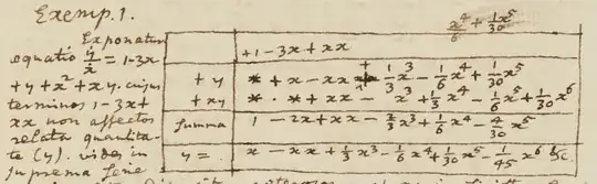
Newton's power series solution of ${dy \over dx} = 1 - 3x + y + x^2 +x y$, with $y(0)=0$ implicitly assumed. Imagine calculating from left to right, column by column, each power of $x$ (what Newton called "the number of dimensions" of $x$). The asterisks denote a missing term, taken to be zero. The terms without $y$ are on top; the series expansions for the terms with $y$ are in the next section. The row labeled "Summa" yields the expansion for $y'$ and the line below is the integral. Once a column has been integrated, one may fill in the next column and integrate again. †Newton's first examples are reversing differential equations obtained by (implicit) differentiation, what we would now call exact equations.