As noted in the comments, identities like this have been mentioned in Modularity of special motives of rank four associated with Calabi-Yau threefolds. Below I sketch the proof of a statement that is slightly more general than yours, namely that for any contour $\gamma$ on $\overline{\mathbb{H}} \setminus j^{-1}(0)$ from one cusp to another one, there are $r^\pm(\gamma) \in \mathbb{Z}^3$ (which we construct explicitly) such that
\begin{align*}
\int_{\gamma} \,
\begin{pmatrix}
1 \\
\tau \\
\tau^2
\end{pmatrix}
\frac{E_4(\tau)}{\sqrt{j(\tau)}} \, \mathrm{d} \tau \, = \, \omega^+ \, r^+(\gamma) + \omega^- \, r^-(\gamma) \, .
\end{align*}
Here, the integrand is understood to be analytically continued along the contour and the numbers $\omega^\pm$ are periods of the unique newform $f \in S_4(\Gamma_0(24))$. In terms of $L$-function values the periods $\omega^\pm$ can be expressed as
\begin{align*}
\omega^+ \, &= \, - \frac{L(f,2)}{(2\pi i)^2} \, = \, 0.0341294416212 \cdots \\
\omega^- \, &= \, -\frac{1}{6} \frac{L(f,1)}{2\pi i} \, = \, 0.0368929462609 \cdots i \, .
\end{align*}
General idea
We consider the hypergeometric function
\begin{align*}
\Pi(z) \, = \, _4F_3\left(\frac{1}{2}, \frac{1}{2}, \frac{1}{6}, \frac{5}{6}; 1, 1, 1; z\right)
\end{align*}
for $0 < z < 1$ and the elementary identities
\begin{align*}
\Pi(z) \, = \, \frac{1}{2\pi i} \oint \frac{1}{\sqrt{1-t}} \, _3F_2\left(\frac{1}{2}, \frac{1}{6}, \frac{5}{6}; 1, 1; \frac{z}{t}\right) \, \frac{\mathrm{d}t}{t} \, =: \, \oint A_{z, 1}(t)
\end{align*}
and
\begin{align*}
\Pi(z) \, = \, \frac{1}{2\pi i} \oint \frac{1}{\sqrt{1-t}} \, _3F_2\left(\frac{1}{4}, \frac{1}{2}, \frac{3}{4}; 1, 1; \frac{2^2}{3^3} \frac{z}{t \, (1-t)^2}\right) \, \frac{\mathrm{d}t}{t} \, =: \, \oint B_{z, 1}(t)
\end{align*}
for suitable contours (e.g. circles counterclockwise around $0$ with fixed radii $|z| < |t| < 1$ for the first and $|t| = 1/3$ for the second). After acting by a monodromy, taking the limit $z \rightarrow 1$ and pulling back by certain modular functions, the first identity will lead to integrals of $E_4/\sqrt{j}$ while the second identity will lead to integrals of the newform $f$.
Because $\Pi$ has the undesired property that it is not holomorphic around $z = 1$, we will consider the linear combination
\begin{align*}
\widetilde{\Pi} \, = \, 4 \, \Pi + M_0 M_1 \Pi \, ,
\end{align*}
where $M_0$ and $M_1$ correspond to the analytic continuation along loops counterclockwise around $0$ and $1$, respectively.
Integrals of $A$
To obtain an integral expression for $\widetilde{\Pi}$, first note that $A_{z, 1}$ is part of a local system of rank three on $\mathcal{M}_z \, = \, \mathbb{P}^1 \setminus \{0,z,1,\infty\}$. We fix some $t_0 > 1$ and choose the following generators of $\pi_1(\mathcal{M}_z, t_0)$:
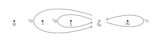
For the local system we can choose a vector of basis elements $A_z$ around $t_0$ such that the first component is $A_{z, 1}$ (with the branch of the square root chosen such that $1/\sqrt{1-t_0} \in i \mathbb{R}_{>0}$) and the monodromy matrices (acting by $A_z \mapsto M_{\gamma} \, A_z$) are given by $M_{\gamma_1} = -T, M_{\gamma_2} = -1, M_{\gamma_3} = S$ in terms of
\begin{align*}
T \, = \,
\begin{pmatrix}
1 & 0 & 0 \\
1 & 1 & 0 \\
1 & 2 & 1
\end{pmatrix}
\qquad \text{and} \qquad
S \, = \,
\begin{pmatrix}
0 & 0 & 1 \\
0 & -1 & 0 \\
1 & 0 & 0
\end{pmatrix}
\, .
\end{align*}
Now consider the map
\begin{align*}
r_z : \ \pi_1(\mathcal{M}_z, t_0) \, &\rightarrow \, \mathbb{C}^3 \\
\gamma \, &\mapsto \, \int_{\gamma} A_z \, .
\end{align*}
It is easy to see that this satisfies the cocycle property $r_z(\gamma \gamma') = r(\gamma) + M_{\gamma} \, r(\gamma')$ and hence it is also completely determined by its values on a set of generators. The analytic continuations in $z$ give the following actions:
\begin{align*}
\begin{array}[h]{c|ccc}
\gamma & \gamma_1 & \gamma_2 & \gamma_3 \\ \hline
M_0 \, r_z(\gamma) & T \, r_z(\gamma_1) & T \, r_z(\gamma_2) & T \, r_z(\gamma_1^{-1}\gamma_2^{-1}\gamma_3\gamma_1\gamma_2^{-1}) \\
M_1 \, r_z(\gamma) & r_z(\gamma_1) & r_z(\gamma_3\gamma_2\gamma_3^{-1}) & r_z(\gamma_3)
\end{array}
\end{align*}
From $\Pi(z) = (1, 0, 0) \cdot r_z(\gamma_1^{-1}\gamma_2^{-1})$ and the analytic continuation we then get
\begin{align*}
\widetilde{\Pi}(z) \, &= \,
\begin{pmatrix}
3 \\ 0 \\ -2
\end{pmatrix}
\cdot r_z(\gamma_1) +
\begin{pmatrix}
-1 \\ 2 \\ 1
\end{pmatrix}
\cdot r_z(\gamma_2) +
\begin{pmatrix}
-2 \\ 0 \\ 0
\end{pmatrix}
\cdot r_z(\gamma_3) \\
&= \,
\begin{pmatrix}
3 \\ 0 \\ -2
\end{pmatrix}
\cdot r_z(\gamma_1) +
\begin{pmatrix}
-3 \\ 2 \\ 1
\end{pmatrix}
\cdot r_z(\gamma_3) \, .
\end{align*}
Here, we used that $(-1,2,1) \cdot r_z(\gamma_2) = (-1,2,1) \cdot r_z(\gamma_3)$ since the integrand is holomorphic around $t = z$ and hence the countour $\gamma_2$ can be pushed outside of the region that gets pinched for $z \rightarrow 1$.
We now restrict to $z = 1$. Then $r_1$ is completely determined by the values on the two generators $\gamma_1$ and $\gamma_3$. Further, we know that $(1,0,1) \cdot r_1(\gamma_3) = 0$ since the integrand is holomorphic around $t = 1$ and hence
\begin{align*}
r_1(\gamma_3) \, = \,\lambda^+ \,
\begin{pmatrix}
-1 \\ 0 \\ 1
\end{pmatrix}
+ \lambda^- \,
\begin{pmatrix}
0 \\ 1 \\ 0
\end{pmatrix}
\end{align*}
for some $\lambda^\pm \in \mathbb{C}$. It is easy to see that in fact $\lambda^+$ must be real while $\lambda^-$ must be purely imaginary. In the limit $t_0 \rightarrow \infty$ these numbers completely determine $r_1$ since then $r_1(\gamma_1) = 0$. In particular, we can then read off $\lambda^\pm$ from
\begin{align*}
\widetilde{\Pi}(1) \, = \, 4 \, \lambda^+ + 2 \, \lambda^- \, .
\end{align*}
As a last step, we consider the modularity of $A$. Pulling back by $t_1 = \frac{1728}{j}$ we get
\begin{align*}
(t_1^*A)(\tau) \, = \, -24\sqrt{3}i \,
\begin{pmatrix}
1 \\
\tau \\
\tau^2
\end{pmatrix}
\frac{E_4(\tau)}{\sqrt{j(\tau)}} \, \mathrm{d}\tau
\end{align*}
around $\tau = \infty$. Every contour $\gamma$ on $\overline{\mathbb{H}} \setminus j^{-1}(0)$ from $\infty$ to a cusp corresponds to an element of $\pi_1(\mathcal{M}_z, t_0)$ (in the limit $t_0 \rightarrow \infty$) and hence the associated integral
\begin{align*}
\int_{\gamma} \,
\begin{pmatrix}
1 \\
\tau \\
\tau^2
\end{pmatrix}
\frac{E_4(\tau)}{\sqrt{j(\tau)}} \, \mathrm{d} \tau
\end{align*}
can be obtained from $r_1$. For example, we have
\begin{align*}
\int_0^\infty \,
\begin{pmatrix}
1 \\
\tau \\
\tau^2
\end{pmatrix}
\frac{E_4(\tau)}{\sqrt{j(\tau)}} \, \mathrm{d} \tau
\, = \, -\frac{1}{-24\sqrt{3}i} \, r_1(\gamma_3)
\, = \, \frac{1}{24 \sqrt{3} i}
\begin{pmatrix}
-\lambda^+ \\
\lambda^- \\
\lambda^+
\end{pmatrix}
\, .
\end{align*}
Integrals of $B$
We proceed analogous to the previous part. $B_{z, 1}$ is part of a local system of rank three on $\mathcal{M}_z = \mathbb{P}^1 \setminus \phi_z^{-1}\{ 0,1,\infty \}$, where $\phi_z(t) = \frac{2^2}{3^3} \frac{z}{t \, (1-t)^2}$. We fix some $t_0 \gg 1$ and choose the following generators of $\pi_1(\mathcal{M}_z, t_0)$:
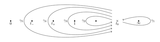
For the local system we can choose a vector of basis elements $B_z$ around $t_0$ such that the first component is $B_{z, 1}$ (with the branch of the square root chosen such that $1/\sqrt{1-t_0} \in i \mathbb{R}_{>0}$) and the monodromy matrices (acting by $B_z \mapsto M_{\gamma} \, B_z$) are given by $M_{\gamma_1} = -T^3, M_{\gamma_2} = -W, M_{\gamma_3} = T^{-1}WT^{-1}, M_{\gamma_4}=-T^{-2}, M_{\gamma_5}=T^{-1}WT^{-1}$ in terms of
\begin{align*}
T \, = \,
\begin{pmatrix}
1 & 0 & 0 \\
1 & 1 & 0 \\
1 & 2 & 1
\end{pmatrix}
\qquad \text{and} \qquad
W \, = \,
\begin{pmatrix}
0 & 0 & 2 \\
0 & -1 & 0 \\
1/2 & 0 & 0
\end{pmatrix}
\, .
\end{align*}
Now consider the map
\begin{align*}
r_z : \ \pi_1(\mathcal{M}_z, t_0) \, &\rightarrow \, \mathbb{C}^3 \\
\gamma \, &\mapsto \, \int_{\gamma} B_z \, .
\end{align*}
The analytic continuations in $z$ give the following actions:
\begin{align*}
\begin{array}[h]{c|ccccc}
\gamma & \gamma_1 & \gamma_2 & \gamma_3 & \gamma_4 & \gamma_5 \\ \hline
M_0 \, r_z(\gamma) & T \, r_z(\gamma_1) & T \, r_z(\gamma_4\gamma_3^{-1}) & T \, r_z(\gamma_4\gamma_2^{-1}) & T \, r_z(\gamma_4) & T \, r_z(\gamma_1^{-1}\gamma_4^{-1}\gamma_5\gamma_1\gamma_4) \\
M_1 \, r_z(\gamma) & r_z(\gamma_1) & r_z(\gamma_2) & r_z(\gamma_3) & r_z(\gamma_5\gamma_4^{-1}\gamma_3) & r_z(\gamma_5)
\end{array}
\end{align*}
From $\Pi(z) = (1, 0, 0) \cdot r_z(\gamma_1^{-1}\gamma_4^{-1})$ and the analytic continuation we then get
\begin{align*}
\widetilde{\Pi}(z) \, &= \,
\begin{pmatrix}
2 \\ 4 \\ -2
\end{pmatrix}
\cdot r_z(\gamma_1) +
\begin{pmatrix}
-1 \\ 0 \\ 0
\end{pmatrix}
\cdot r_z(\gamma_2) +
\begin{pmatrix}
5 \\ 8 \\ 2
\end{pmatrix}
\cdot r_z(\gamma_4) +
\begin{pmatrix}
-1 \\ 0 \\ 0
\end{pmatrix}
\cdot r_z(\gamma_5) \\
&= \,
\begin{pmatrix}
2 \\ 4 \\ -2
\end{pmatrix}
\cdot r_z(\gamma_1) +
\begin{pmatrix}
-1 \\ 0 \\ 0
\end{pmatrix}
\cdot r_z(\gamma_2) +
\begin{pmatrix}
4 \\ 8 \\ 2
\end{pmatrix}
\cdot r_z(\gamma_5) \, .
\end{align*}
Here, we used that $(5,8,2) \cdot r_z(\gamma_4) = (5,8,2) \cdot r_z(\gamma_5)$ since the integrand is holomorphic around $t_{\pm}$ and hence the countour $\gamma_4$ can be pushed outside of the region that gets pinched for $z \rightarrow 1$.
As a last step, we consider the modularity of $B$. For this, consider the modular function
\begin{align*}
t_2(\tau) \, = \, \frac{(\eta(2\tau)/\eta(\tau))^{24}}{(1+64 \, (\eta(2\tau)/\eta(\tau))^{24})^2}
\end{align*}
and the modular function $t_{72}$ which solves $\phi_1(t_{72}(\tau)) = 256 \, t_2(6\tau)$ and has the Fourier expansion $t_{72}(\tau) = \frac{1}{12}q^{-2}+O(q^0)$. Pulling back by $t_{72}$ we get
\begin{align*}
(t_{72}^*B)(\tau) \, = \, -4\sqrt{3}i \,
\begin{pmatrix}
1 \\
6\tau \\
(6\tau)^2
\end{pmatrix}
(f(\tau)-9 \, f(3\tau))\, \mathrm{d}\tau
\end{align*}
around $\tau = \infty$. For $z = 1$ we thus get
\begin{align*}
\widetilde{\Pi}(1) &= \lim_{t_0 \rightarrow \infty} \left(
\begin{pmatrix}
-1 \\ 0 \\ 0
\end{pmatrix}
\cdot r_z(\gamma_2) +
\begin{pmatrix}
4 \\ 8 \\ 2
\end{pmatrix}
\cdot r_z(\gamma_5)
\right) \\
&= -4\sqrt{3}i \left(
\begin{pmatrix}
-1 \\ 0 \\ 0
\end{pmatrix}
\int_{\infty}^0
\begin{pmatrix}
1 \\
6\tau \\
(6\tau)^2
\end{pmatrix}
(f(\tau)-9 \, f(3\tau)) \mathrm{d}\tau
+
\begin{pmatrix}
4 \\ 8 \\ 2
\end{pmatrix}
\int_{\infty}^{-1/6}
\begin{pmatrix}
1 \\
6\tau \\
(6\tau)^2
\end{pmatrix}
(f(\tau)-9 \, f(3\tau)) \mathrm{d}\tau
\right)
\end{align*}
and it is a straightforward exercise in period polynomials to show that the latter evaluates to $-24\sqrt{3}i \, (4\, \omega^- + 2 \, \omega^+)$.
Final steps
In our study of the integrals of $A$ we have constructed $r^\pm(\gamma) \in \mathbb{Z}^3$ such that
\begin{align*}
\int_{\gamma} \,
\begin{pmatrix}
1 \\
\tau \\
\tau^2
\end{pmatrix}
\frac{E_4(\tau)}{\sqrt{j(\tau)}} \, \mathrm{d} \tau \, = \, \frac{1}{-24\sqrt{3}i} \left(\lambda^- \, r^+(\gamma) + \lambda^+ \, r^-(\gamma) \right) \, ,
\end{align*}
where $\lambda^+ \in \mathbb{R}$ and $\lambda^- \in i\mathbb{R}$ are given by $\widetilde{\Pi}(1) = 4\, \lambda^+ + 2 \, \lambda^-$. In our study of the integrals of $B$ we have further shown that
\begin{align*}
\widetilde{\Pi}(1) = -24\sqrt{3}i \, (4\, \omega^- + 2 \, \omega^+)
\end{align*}
with the periods $\omega^\pm$ of $f$. Hence $\lambda^\pm = -24\sqrt{3}i \, \omega^\mp$, which finishes the proof. Note that, by evaluating other analytic continuations and derivatives of $\Pi$ at $z=1$, one can get further identities e.g. featuring quasiperiods of $f$.


